Valuation models for equity indexes are essential tools for investors seeking to assess long-term market conditions. Traditional models like the CAPE ratio, introduced by Robert J. Shiller, or the Buffett Indicator often rely on macroeconomic variables such as corporate earnings or GDP. While informative, these models can be complex and dependent on data that may be revised or vary across regions. In this article, we introduce a simpler alternative: a valuation ratio based solely on the inflation-adjusted total return of the index, offering a streamlined and transparent approach to index valuation. Finally, our goal would be to answer the question from the title – Are the indexes fairly priced at the moment?
Introduction
Our simple, price-based absolute valuation measure is calculated as the difference between the inflation-adjusted Total Return Index (TR Index) and its 30-year moving average. Using historical U.S. market data from 1871 to 2025, we group valuation levels into percentiles and examine their relationship with future return expectations and downside risk over 3-, 5-, and 10-year horizons. The analysis shows that lower starting valuations are generally associated with higher and more stable future returns, while higher valuations increase the likelihood of lower returns and deeper drawdowns, and even overvalued markets can deliver strong returns if conditions are favorable. We also compare two types of drawdowns (maximum drawdown from time of investment and rolling maximum drawdown), both of which highlight increasing risk at higher valuation levels. Currently, the TR Index stands at 146% of its 30-year moving average, placing the market in the 60th–70th percentile range. This suggests a moderately overvalued market.
Theory
Absolute valuation measures are tools used to assess whether a stock market or asset is overvalued or undervalued based on its own fundamentals. Common measures include the Price-to-Earnings (P/E) ratio; the Price-to-Book (P/B) and Price-to-Sales (P/S) ratios, which relate prices to book value or revenues; and the Dividend Yield, which indicates how much income investors receive relative to price. One widely used metric is CAPE (Cyclically Adjusted Price-to-Earnings ratio), developed by Robert J. Shiller, which smooths earnings over a 10-year period to reduce the impact of business cycle fluctuations and provide a more stable view of market valuation. Another influential indicator is the Buffett Indicator, popularized by Warren Buffett, which compares the total market capitalization of publicly traded equities to a country’s GDP and is often interpreted as a broad measure of whether the stock market is overvalued relative to the overall economy. Other indicators include the Earnings Yield (the inverse of P/E), Tobin’s Q (market value vs. replacement cost of assets), and the Implied Equity Risk Premium, which reflects expected returns over the risk-free rate. These measures are often used to explore the link between market valuation and future returns.
All of the above valuation measures share a common structure: their numerator is always based on the current value of the stock market. The numerator is usually volatile and responsive to short-term market fluctuations. On the other hand, the denominator typically reflects a slow-moving variable (such as GDP or 10-year cyclically adjusted earnings), which evolves gradually over time. Even though many valuation measures exist, if the market is truly overvalued on an absolute basis, they will all signal overvaluation. In other words, they tend to differ not in direction (whether the market is overvalued), but in magnitude (how much overvalued it is). While each measure may offer a different estimate of expected future returns over 3, 5, or 10 years, the variability between these estimates is typically minor. For example, a predicted return of 5% from one measure versus 7% from another does not represent a meaningful divergence. Given this, if an approximate forecast is sufficient, price-based valuation measures can be used for predictive purposes, simplifying the overall approach.
All of these measures have their own advantages and limitations, and our goal is not to determine which is best. Instead, in this article, we propose and test a simple price-based absolute valuation measure to analyze how the level of overvaluation of the stock market on an absolute basis affects future risk and returns.
Methodology & Data
For our analysis, we use the dataset provided by Robert J. Shiller, available at shillerdata.com, which includes long-term historical data on U.S. stock market valuation, earnings, and interest rates. Dataset spans from January 1871 to March 2025.
First, we created Total Return Index (TR Index) as change in the price of stocks plus dividend paid (divided by 12) to approximate monthly return. Then, we calculated inflation adjusted TR Index using the Consumer Price Index (CPI) as a monthly change in the TR Index minus the monthly change in CPI. After calculating the Total Return Index and its inflation adjusted counterpart, we plotted the results on a logarithmic scale (Figure 1). The slope of the trend line, representing the long-term average real return, is approximately 4% annually. This long-term average serves as a historical benchmark. All absolute valuation measures generally follow the principle of mean reversion. If market returns have exceeded this average in recent years, it is likely that future growth will slow in order to revert toward the historical trend.
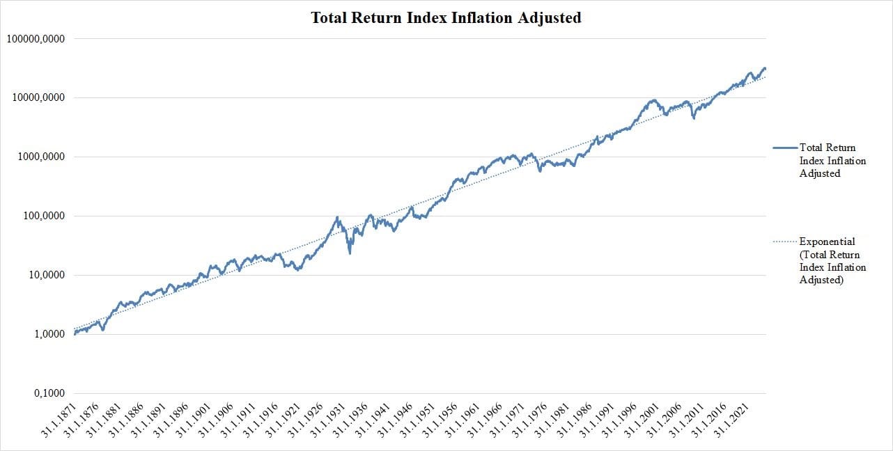
Figure 1 Inflation-Adjusted Total Return Index with Long-Term Trend
However, we recognize that using a regression over 150 years of data as an absolute valuation predictor may not be methodologically correct. This kind of analysis uses future returns to evaluate current valuations, which can lead to biased results. To address this, we introduce a more flexible benchmark: the 30-year price moving average. In Figure 2, we plot both the inflation adjusted Total Return Index and its 30-year moving average. This moving average is intended to represent a more realistic valuation anchor with 30 years roughly corresponding to one generation of investors.
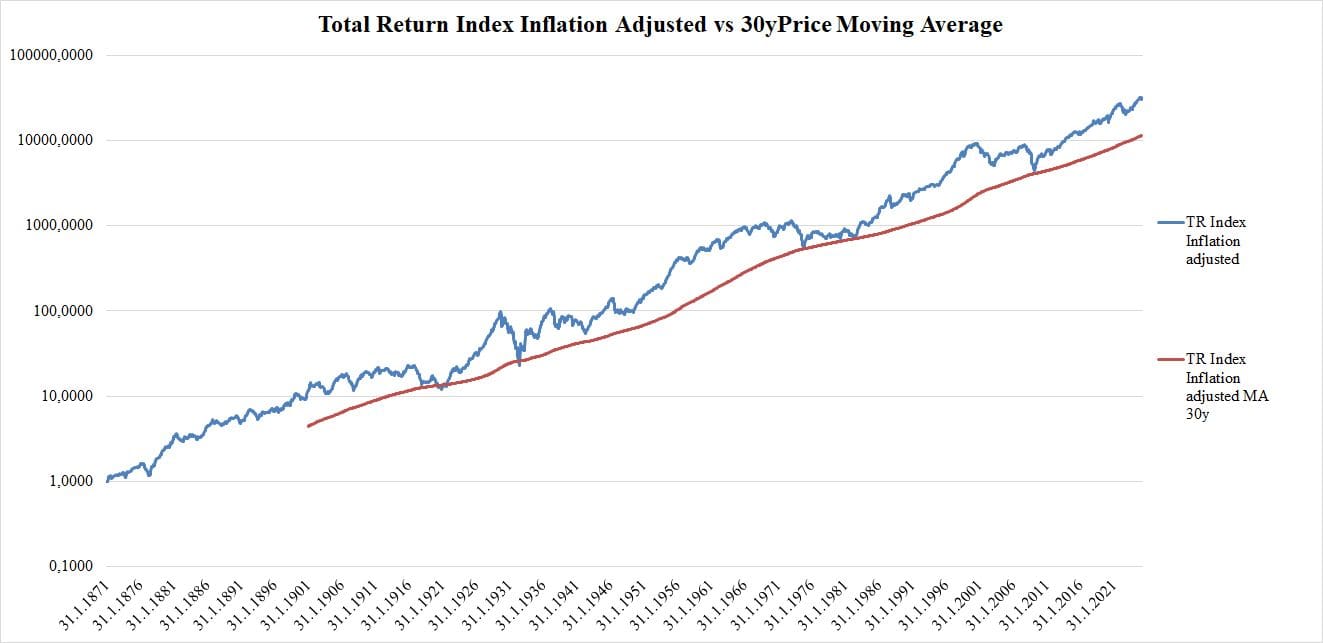
Figure 2 Inflation-Adjusted Total Return Index vs. 30-Year Moving Average
Following the structure of other absolute valuation measures, our approach also includes one quickly-moving variable in the numerator (Inflation Adjusted Total Return Index) and one slowly-moving variable in the denominator (constructed simply as the 30-year moving average of the Inflation Adjusted Total Return Index). By comparing the current market level to this slowly evolving baseline, we propose a simple valuation approach based on the relationship between price and its long-term trend. This method provides an approximate forecast of potential future returns.
Next, in our analysis we focused on how valuation affects risk and return. We first calculated 11 percentile ranges based on the degree of market overvaluation, measured as the difference between the Inflation Adjusted Total Return Index and its 30-year moving average. For each of these valuation groups, we computed return scenarios over 3-, 5-, and 10-year horizons, using the 10th and 25th percentiles as pessimistic cases, the 50th percentile as the realistic (median) case, and the 75th percentile as an optimistic case. For risk, we evaluated two types of drawdowns: max drawdown from time of investment (shown in purple in Figure 3) and rolling max drawdown (shown in red in Figure 3). For both drawdown types, we applied the same structure as for returns, calculating the 10th, 25th, 50th, and 75th percentile values across each valuation group and investment horizon.
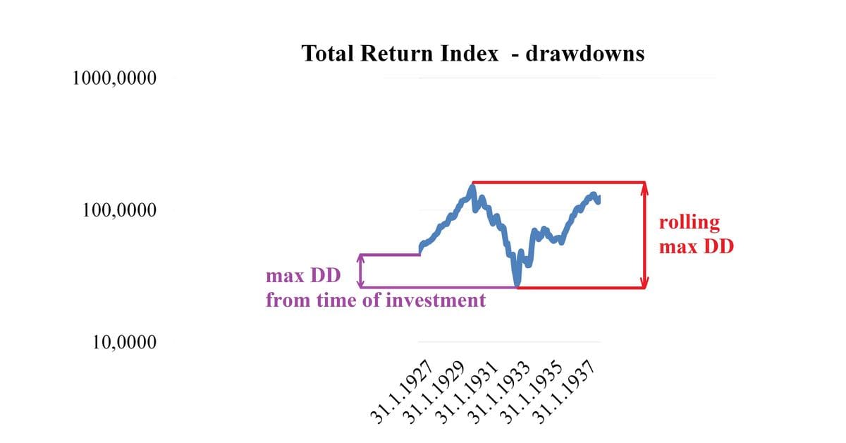
Figure 3 llustration of two drawdown types. The purple arrow shows the maximum drawdown from the time of investment. The red arrow shows the rolling maximum drawdown during the 10y investment period
Results
Returns
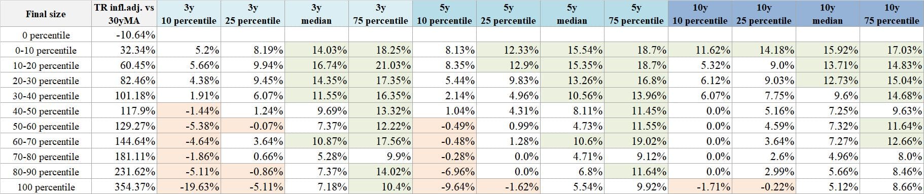
Table 1 Total Returns by Valuation Percentile (TR Index vs. 30-Year Moving Average) for 3-, 5-, and 10-Year Periods
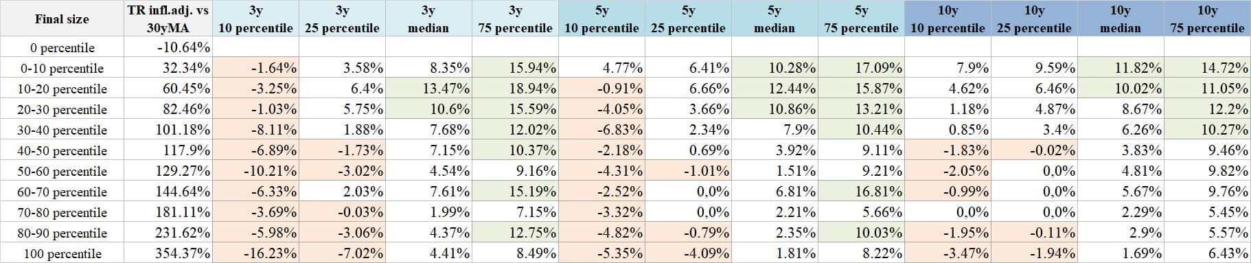
Table 2 Inflation-Adjusted Total Returns by Valuation Percentile (TR Index vs. 30-Year Moving Average) for 3-, 5-, and 10-Year Periods
Even when the market is overvalued, you can still earn positive short-term returns.
When the market is in the highest valuation percentiles (TR Index vs. 30-year moving average in the 80th–100th percentile range, see Table 1), the 75th percentile of 3-year forward returns remains positive—around 10–14%. This means that under favorable conditions, even expensive markets can deliver decent short-term gains. The same holds true for inflation adjusted returns (see Table 2).
Starting valuation affects long-term returns.
When the market is in the lowest valuation percentiles (TR Index vs. 30-year moving average in the 0–10 percentile range, see Table 1), the median 10-year return is around 15%. In contrast, when the market is in the highest valuation percentile (100th), the median 10-year return drops to around 5%. This pattern also appears in inflation adjusted returns (see Table 2).
Short-term returns are more variable and depend on luck.
At low valuations (TR Index vs. 30-year moving average in the 0–10 percentile range, see Table 1), 3-year returns range from about 5% (10th percentile) to 18% (75th percentile). At high valuations (100th percentile), they range from -19,6% to around 10,4%. This wide spread shows that short-term outcomes are uncertain, but valuation still shifts the odds.
However, even in short-term, lower valuations improve the odds of attractive returns.
Across all percentiles, 3-year returns are consistently higher in low-valuation groups than in high-valuation ones. For example, the 3-year median return in the 0–10th percentile valuation group is 14.0%, compared to just 7.2% in the 90–100th percentile group.
Risk
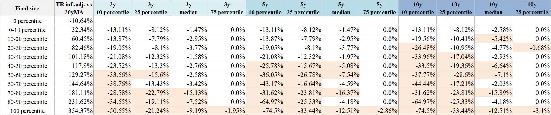
Table 3 Maximum Drawdown from Time of Investment by Valuation Percentile (TR Index vs. 30-Year Moving Average) for 3-, 5-, and 10-Year Periods
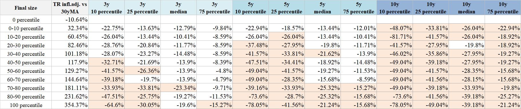
Table 4 Rolling Maximum Drawdown by Valuation Percentile (TR Index vs. 30-Year Moving Average) for 3-, 5-, and 10-Year Periods
The level of valuation (as measured by TR Index vs. 30-year MA) doesn’t just predict future returns—it also affects the distribution of potential losses. In other words, higher valuations come with higher risk, not just lower expected returns.
At high valuations, the chance of negative returns is significant—at low valuations, it is minimal.
As seen in Table 3, when valuations are high (80th–100th percentile), the 10th percentile of 3-, 5-, and 10-year returns drops below -30%, even down to -50% or worse. In contrast, at low valuation levels, this downside risk is noticeably reduced.
Higher valuation increases the risk of sharp drawdowns, even if the investment ends up profitable.
Tables 3 and 4 illustrate Max DD from the time of investment and rolling max DD. At high valuations, investors are more likely to experience significant declines during the investment period, making the road bumpy – more volatile and stressful, even if the end result is positive.
Some tail risk (especially over longer horizons) is non-diversifiable.
For 10y horizon, At the 10th percentile, drawdowns across all valuation levels are -45% or worse (see Table 3). Over long periods, “once-in-a-generation” events such as the Great Depression (1930s) or Global Financial Crisis (2008) are plausible. Every investor should be aware of this and be mentally prepared to face such outcomes.
One might wonder, where are we now?
As of April 30th 2025, the inflation-adjusted Total Return Index relative to its 30-year moving average stood at 146%. Referring back to Table 1 and Table 2, this value places the market in the 60th–70th percentile range. This means the market is more overvalued than at least 60% of historical observations. At the current valuation level, expected median returns range from 10.9% over 3 years to 7.3% over 10 years (nominal), or 7.6% (3y) to 5.7% (10y) when adjusted for inflation. Risk remains moderate, with maximum drawdowns from the time of investment under 5% in the median case, but rolling drawdowns reaching -8.6% to -28.1% (10y).
To put the current valuation into perspective:
On December 31, 2007, just before the Global Financial Crisis, the inflation-adjusted Total Return Index stood at 122% of its 30-year moving average, placing the market in the 50th–60th percentile. Today, we are in a comparable situation, just slightly above the 2007 pre-crisis level. Stock prices have declined, but they are still not historically cheap.
On December 31, 1999, at the peak of the dot-com bubble, the index reached 327% of its 30-year moving average, placing it in the highest historical percentile and signaling extreme overvaluation.
In contrast, on March 31, 2009, near the bottom of the Global Financial Crisis, the valuation index fell to just 9% of its 30-year moving average. This placed the market in the lowest historical percentiles, indicating a period of clear undervaluation and strong long-term investment potential.
Conclusion
In this article we introduced a simple absolute valuation measure based on the difference between the inflation adjusted Total Return Index and its 30-year moving average. Using this measure, we grouped market valuations into percentile ranges and analyzed future return expectations and associated risks over 3-, 5-, and 10-year horizons.
Our analysis shows that markets starting from lower valuation levels tend to deliver higher and more stable returns. However, strong returns are still possible even when the market is overvalued, if conditions are favorable. At the same time, high valuation levels are associated with increased risk. Some risks, particularly over longer horizons are unavoidable, as extreme market events can occur regardless of starting valuation. As of April 2025, the market was moderately overvalued compared to its long-term trend. Although stock prices have declined recently, they are still not cheap, so investors should keep their expectations modest.
Author: Margareta Pauchlyova, Quant Analyst, Quantpedia
Are you looking for more strategies to read about? Sign up for our newsletter or visit our Blog or Screener.
Do you want to learn more about Quantpedia Premium service? Check how Quantpedia works, our mission and Premium pricing offer.
Do you want to learn more about Quantpedia Pro service? Check its description, watch videos, review reporting capabilities and visit our pricing offer.
Are you looking for historical data or backtesting platforms? Check our list of Algo Trading Discounts.
Would you like free access to our services? Then, open an account with Lightspeed and enjoy one year of Quantpedia Premium at no cost.
Or follow us on:
Facebook Group, Facebook Page, Twitter, Linkedin, Medium or Youtube